Predict future price in Polish stock exchange using Tensorflow and Jupyter Notebooks

Recently, I’m a bit fascinated by the stock market and I thought that I would combine my two passions and work a bit more on predicting the price of shares using neural networks. The model of the network that works to solve such a problem is the RNN model, which allows you to predict the value of the next step by analyzing the current one. I found a wonderful blog post writed by Lilian Weng with a description of a model that works well with the prediction of the American stock market. To use the Lilian code I decided to make a few changes and introduce some facilities such as:

• The code was not prepared to work with Python version 3 and I had to adjust it to work with this version. I just prefer Python 3 and I think evertyhing new that is create should be write with newest version ;).
• I wanted to use Jupyter notebooks so that I could easily examine changes in my code and customize it on a regular basis.
• I love to use Docker projects so that I can easily move them between my computers.
• It is difficult to find stock market data of the Polish stock exchange (at least for free).
• Lilian use Yahoo! Finance data and it’s a bit different than data which I found for Polish exchange.

In the first place I wanted to find a suitable container with Jupyter Notebooks and Tensorflow. In addition, I wanted to be able to analyze the work of Tensorflow session using the built-in Tensorboard and it turned out that there is a plugin for Jupyter Notebooks that allows you to enter the Tensorboard from the notebook. It can be found at Shengpend Liu GitHub but to be able to use Tensorboard, you still have to install the tensorflow-tensorboard library in a container. I create my own Dockerfile to fix this issue:

from lspvic/tensorboard-notebook
RUN pip install tensorflow-tensorboard

I started the above image with the MongoDB image (future use) using docker-compose. This is docker-compose.yml which I use:

version: '3'
services:
  jupyter:
    build: ./jupyter_tensorflow_tensorboard/
    ports:
      - "8888:8888"
    volumes:
      - ./notebooks:/home/jovyan/work/
  mongo:
    image: mongo
    ports:
      - "27017:27017"

One thing to keep in mind is giving the right permissions to the directory (mounted) which will be used to save your work. I gave it full access using the command:

chmod 777 -R ./notebooks

The next step was to find data from the Polish stock exchange. I found them on the site of BOSSA.pl. It is one of the most modern Polish brokers also having API for stock exchange transactions (as one of few, or even the only one on the Polish market). Data consists of daily opening, closing, top prices and volume and reach back to 1991 (the beginning of the stock exchange in Poland - yes it’s so young). I also added a code element that allows downloading current stock data, but only if its not downloaded already today (they update daily). The data includes the prices of all companies listed on the Warsaw Stock Exchange, but for the time being I only use the prices of WIG shares to train model. (you can use few or all of them, just read Lilian blog to learn how to).

The last step and the most important was to adapt the Lilian code to Python 3 and launch the training and testing process in Jupyter Notebook. I use few Python scripts from Stock-RNN project which I adapt to work with data from BOSSA.pl and version 3 of Python. Part of the code responsible for preparing the whole project:

import os
import numpy as np
import pandas as pd
import random
import time
from datetime import datetime
import tensorflow as tf
import tensorflow.contrib.slim as slim
from io import BytesIO
from zipfile import ZipFile
from urllib.request import urlopen
import matplotlib.pyplot as plt
from stock_rnn.scripts.build_graph import build_lstm_graph_with_config
from stock_rnn.scripts.train_model import train_lstm_graph
from stock_rnn.scripts.restore_model import prediction_by_trained_graph
from stock_rnn.scripts.config import DEFAULT_CONFIG, MODEL_DIR
from stock_rnn.data_model import StockDataSet

DATA_DIR = "stock_data"
NEW_DATA_DIR = "new_stock_data"
BOSSA_PL_STOCK_DATA_URL = "http://bossa.pl/pub/metastock/mstock/mstall.zip"
WIG_PATH = os.path.join(DATA_DIR, "WIG.mst")
TRAINING_MODEL_STOCK = "WIG"

#Simple method to plot prediction results in compare to data sample 
def plot_samples(preds, targets, stock_sym=None, multiplier=5):
        def _flatten(seq):
            return np.array([x for y in seq for x in y])

        truths = _flatten(targets)[-200:]
        preds = (_flatten(preds) * multiplier)[-200:]
        days = range(len(truths))[-200:]

        plt.figure(figsize=(12, 6))
        plt.plot(days, truths, label='truth')
        plt.plot(days, preds, label='pred')
        plt.legend(loc='upper left', frameon=False)
        plt.xlabel("day")
        plt.ylabel("normalized price")
        plt.ylim((min(truths), max(truths)))
        plt.grid(ls='--')

        if stock_sym:
            plt.title(stock_sym + " | Last %d days in test" % len(truths))
            
#Just to preview data
df_wig = pd.read_csv(WIG_PATH)
df_wig['<OPEN>'].plot()

You can configure model changing parameters of DEFAULT_CONFIG, please check stock_rnn/scripts/config.py for whole list of parameters. When you ran this part of notebook you can see WIG stock price plotted - it simple tells you that data is on its place. I added the data directory in case they were not available at BOSSA.pl at one time but at the time of writing this post fresh data are availible every day and you can download it using second notebook cell:

#Download newest stock data if not downloaded today and unzip
today = datetime.now()
today_dir = os.path.join(NEW_DATA_DIR, today.strftime('%Y%m%d'))

if(not os.path.exists(today_dir)): 
   os.makedirs(today_dir)
   resp = urlopen(BOSSA_PL_STOCK_DATA_URL)
   zipfile = ZipFile(BytesIO(resp.read()))
   zipfile.extractall(today_dir)

Now it’s time to build and train model:

#Build graph and train it for stock symbol provided
lstm_graph = build_lstm_graph_with_config(config=DEFAULT_CONFIG)
train_lstm_graph(TRAINING_MODEL_STOCK, lstm_graph, config=DEFAULT_CONFIG)

You can configure stock symbol to train with using TRAINING_MODEL_STOCK variable. After while (or more) model is trained and saved. You can easily test it with other stock prices data:

#Load trained graph and test on other stock data (or same)
TEST_MODEL_STOCK = "WIG20"

stock_data_set =  StockDataSet(
   TEST_MODEL_STOCK,
   input_size=1,
   num_steps=30,
   test_ratio=1.0)

Here I just use StockDataSet to create test data from downloaded stock price data files. test_ratio param is set to 1.0 because all data will be used as test data (class is originally build to create, train and test data with provided ratio). Now its time to test:

#Load graph trained in previous step
graph_name = "%s_lr%.2f_lr_decay%.3f_lstm%d_step%d_input%d_batch%d_epoch%d" % (
        TRAINING_MODEL_STOCK,
        DEFAULT_CONFIG.init_learning_rate, DEFAULT_CONFIG.learning_rate_decay,
        DEFAULT_CONFIG.lstm_size, DEFAULT_CONFIG.num_steps,
        DEFAULT_CONFIG.input_size, DEFAULT_CONFIG.batch_size, DEFAULT_CONFIG.max_epoch)
test_prediction, test_loss = prediction_by_trained_graph(graph_name, DEFAULT_CONFIG.max_epoch, stock_data_set.test_X, stock_data_set.test_y)

Pay attention to the name of graph (graph_name variable) because it needs to be same as graph saved during training process. If you don’t change DEFAULT_CONFIG beetween traing and testing then grap_name variable should be OK. Last but not least we can plot our prediction:

plot_samples(test_prediction, stock_data_set.test_y, TEST_MODEL_STOCK)

I just use Lilian method but with small changes which allow to plot in Jupyter. If everything is ok you should see result like this:

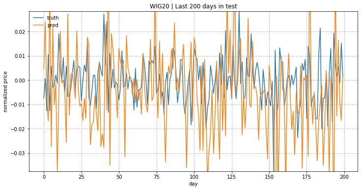
Please remember that price move is normalized and it’s showing relative change rates instead of the absolute values!

This is it! You can find whole project in my GitHub account and I strongly suggest that you read the great work of Lilian.

Please remember that the price prediction of stock exchange shares is very difficult and requires a much richer model and a larger amount of data. Thanks for reading!